Historical Volatility vs. Implied Volatility: An In-depth Analysis

Volatility is the key to profit. While this holds a bit for investors with higher risk appetite, the conservative ones provocatively deny this statement. Do you know why? They simply don’t know how to utilize volatility metrics to strategically set up take-profit levels. 

This article will explore the concepts of historical and implied volatility. We will begin by understanding historical volatility and the process of calculating it using standard deviation. We will then go through a practical example of this calculation for a stock over a 30-day period. Also, we’ll discuss the significance of historical volatility in assessing market sentiment and risk. 

Next, we’ll explain implied volatility, how it’s derived from options prices, and its role in forecasting future price movements. Moreover, we’ll compare historical and implied volatility, including strategies like volatility arbitrage, and how traders use straddle and strangle options strategies. 

Finally, we’ll show how volatility metrics help determine position sizes and set stop-loss and take-profit levels to manage risk effectively. Let’s get started.

What is Historical Volatility? 

Historical volatility shows the amount by which an asset’s price has fluctuated over a given period in the past. Traders and investors often use this metric to gauge the risk associated with an asset. 

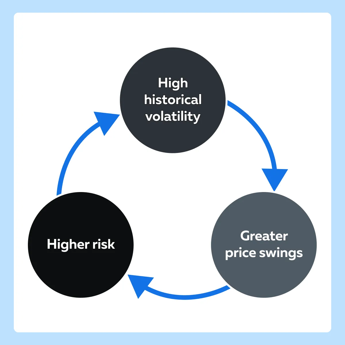
As per a thumb rule, the higher the historical volatility, the greater the price swings, signaling increased risk for traders and investors. Conversely, lower historical volatility indicates more stable prices and predictable prices, often preferred by those with a lower risk tolerance.

How to Calculate Historical Volatility

You can calculate historical volatility using several online calculators. They simplify the process of calculating by requiring you to input some basic data. Let’s study some simple steps that help you calculate historical volatility for a stock over a 30-day period using an online calculator:

• Gather Historical Price Data
  • Obtain the closing prices for the stock over the past 30 trading days.
  • You can get this data from the stock’s historical data page or from financial websites like Yahoo Finance and Google Finance.
• Choose an Online Calculator:
  • Search for an online historical volatility calculator.
  • Some popular options include calculators provided by Investopedia, MarketWatch, or specialized financial analytics websites.
• Input the Data
  • Open the calculator and enter the 30 days of closing prices.
  • Some calculators might ask for daily returns instead of prices, in which case you can enter the percentage change in price from one day to the next.
• Calculation Process
  • The calculator will perform the following calculations internally:
    • Calculate the daily returns.
    • Determine the average of the daily returns.
    • Subtract the average return from each daily return and square the result.
    • Find the average of these squared differences.
    • Take the square root of this average to get the standard deviation, which represents the historical volatility.
• Obtain the Result
  • After you input the required data, the calculator will provide the historical volatility as a percentage.
  • This represents the annualized standard deviation of the stock’s daily returns over the 30-day period.

Let’s go through an example where we calculate the historical volatility of a stock over a 30-day period.

• Assume you found out the closing prices for the past 30 days.
• Now, you decided to use an online calculator, such as the one on Investopedia.
• You entered the 30 closing prices into the calculator.
• The calculator computes the daily returns based on the input prices.
• It calculates the standard deviation of these daily returns.
• The calculator outputs the historical volatility, for instance, 2.5%.
• This means that over the past 30 days, the stock’s price has fluctuated with an annualized volatility of 2.5%.

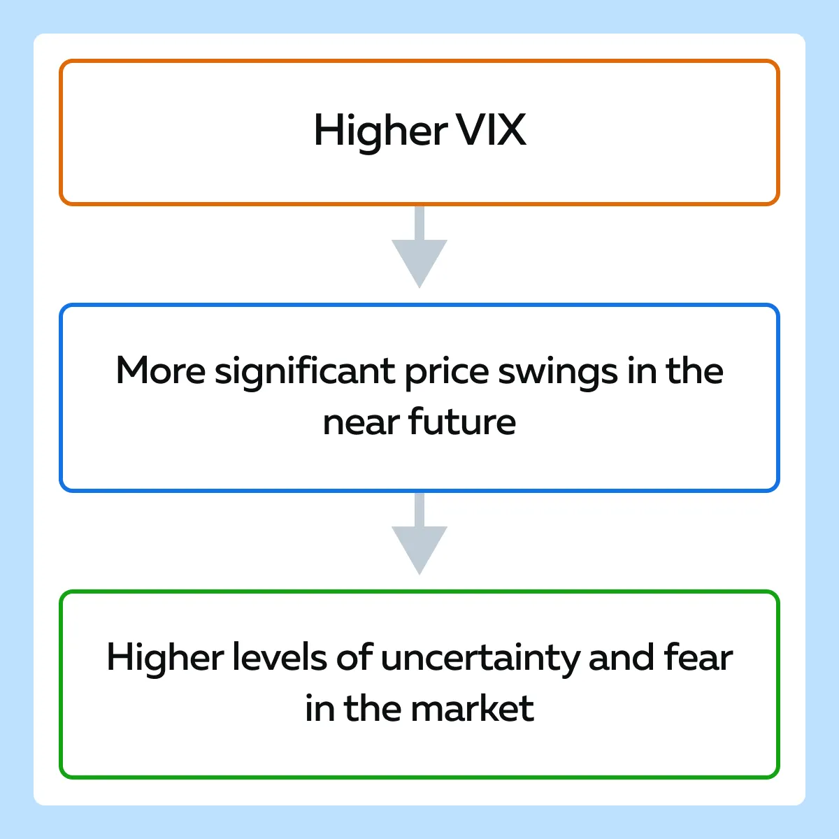
The concept of historical volatility is closely associated with the VIX or Volatility Index. It is often referred to as the “fear gauge” of the market. Let’s study in detail:

What is VIX?

It measures the market’s expectation of 30-day volatility. VIX is derived from the prices of S&P 500 index options. Traders must note that VIX is a forward-looking measure. It is different from historical volatility, which looks at past price movements. While historical volatility is calculated using past data, the VIX uses options pricing to reflect investors’ expectations of future volatility. 

 

Significance of Historical Volatility 

Historical volatility shows how an asset’s price has behaved over a specific period. It reflects past market sentiment and price behavior by quantifying the degree of price fluctuations. 

High historical volatility	Low historical volatility
It indicates that an asset’s price has experienced large swings. It suggests a period of uncertainty or significant market events.	It signals stable prices and a calmer market environment.

 

By examining historical volatility, traders can gain insights into the:

• Historical risk 

and

• Stability of an asset.

 

This information is valuable for understanding how an asset might react to future market conditions based on its past performance.

How Do Traders Assess Risk Via Historical Volatility?

Historical volatility provides a numerical measure of the risk. It is noteworthy to state that assets with higher historical volatility are considered riskier because their prices have shown greater variability. 

Furthermore, by understanding the volatility of different assets, traders can diversify their portfolios to balance:

• Risk

and

• Rewards.

Historical volatility is also a crucial input in option pricing models like the Black-Scholes model. Traders use it to estimate the fair value of options and strategize hedging techniques.

Let’s understand this better using a scenario where historical volatility is used to determine the risk level of a tech stock:

The scenario

• Say a trader evaluates the risk of investing in a tech stock, XYZ Corp.
• The trader collects the daily closing prices of XYZ Corp for the past 30 days.
• The trader calculates the daily returns based on these closing prices.
• These daily returns’ mean and standard deviation are computed to determine the historical volatility.
• Suppose the trader finds that XYZ Corp has high historical volatility compared to other stocks in the same sector.
• This high volatility suggests that XYZ Corp’s stock price has experienced significant fluctuations in the past month, indicating higher risk.

 

Risk assessment

• The trader notes that the high historical volatility is due to recent:
  • Tech industry news,
  • Earnings reports, or
  • Broader market movements affecting tech stocks.
• The trader considers that past price behavior reflects market sentiment.
• It possibly indicates that investors are uncertain about the future performance of XYZ Corp.

Investment decision

• • The trader assesses their own risk tolerance.
  • If they are a risk-averse investor, they can decide to avoid investing in XYZ Corp due to its high volatility.

• If the trader has a higher risk tolerance, they might see the high volatility as an opportunity for potentially higher returns.

 

Comparison with VIX

• The trader also looks at the VIX to gauge broader market expectations of volatility.
• If the VIX is high, it indicates that the market anticipates higher volatility, which could further impact the tech sector.

What is Implied Volatility? 

Implied volatility (IV) is the market’s forecast of a likely movement in an asset’s price. It is derived from the price of options and reflects the market’s expectations of future volatility. Unlike historical volatility, which looks at past price movements, implied volatility is forward-looking. It is influenced by the following factors:

• Market sentiment,
• Upcoming events, and 
• Overall market conditions.

 

To better understand implied volatility, let’s consider an example involving a tech company, ABC Corp, which is about to release its quarterly earnings report.

The scenario

• Traders are anticipating that ABC Corp will report strong earnings.
• Before the earnings announcement, many traders expect significant price movements.
• Some traders may want to capitalize on potential price increases, while others may want to hedge against potential declines.

As a result of this anticipation

• There is increased trading activity in ABC Corp’s options.
• More traders buy call options (betting on a price increase) and put options (betting on a price decrease or hedging).
• This increased trading activity leads to a higher demand for these options.
• The increased demand for options drives up their prices.
• Higher option prices imply greater expected volatility, causing the implied volatility to spike.

Putting in numbers

Pre-Earnings Period	Earnings Anticipation	Post-Earnings
One week before the earnings release, the implied volatility of ABC Corp’s options is 25%.	As the earnings announcement approaches, traders speculate on potential significant price movement. This drives implied volatility up to 40%.	After the earnings report is released, the uncertainty is resolved. If the earnings meet expectations, implied volatility might decrease back to around 25%.  If earnings surprise (either positively or negatively), implied volatility will adjust based on the new information and market reaction.

 

How to Calculate Implied Volatility?

Implied volatility is calculated using options pricing models like the Black-Scholes model. This model uses several inputs to estimate the fair value of an option, one of which is the implied volatility. Below are some inputs required for the calculation purposes:

• Current Stock Price (S): The current price of the underlying asset
• Strike Price (K): The price at which the option can be exercised
• Time to Expiration (T): The time remaining until the option’s expiration date, expressed in years
• Risk-Free Rate (r): The risk-free interest rate, typically based on government bonds
• Implied Volatility (σ): The expected volatility of the asset’s price over the life of the option

Assume we have the following data for ABC Corp:

• Current Stock Price (S): $100
• Strike Price (K): $105
• Time to Expiration (T): 0.25 years (3 months)
• Risk-Free Rate (r): 2% (0.02)
• Options Price (C): $5

Now, you can apply the Black-Scholes formula for a call option using any online calculator. It must be noted that in practice, calculating implied volatility involves:

• Using the known option price ($5 in this case) 

and

• Iteratively adjust the implied volatility (σ) until the Black-Scholes model price matches the market price of the option.

 

Let’s see how you can do so by following these simple steps:

• Guess Initial σ: Start with an initial guess for implied volatility.
• Calculate Option Price: Use the Black-Scholes formula to calculate the option price with the guessed σ.
• Compare Prices: Compare the calculated option price with the market price ($5).
• Adjust σ: Adjust the implied volatility guess up or down based on whether the calculated price is lower or higher than the market price.
• Iterate: Repeat steps 2-4 until the calculated option price converges to the market price.

Significance of Implied Volatility 

Implied volatility (IV) reflects the market’s expectations of future price volatility for an asset. Unlike historical volatility, which is based on past price movements, implied volatility:

• Is derived from the market prices of options

and

• Indicates how much the market believes an asset’s price will fluctuate in the future.

 

Usually, high implied volatility suggests that the market expects significant price movements. This happens due to several upcoming events, such as:

• Earnings reports,
• Economic data releases, or
• Geopolitical developments.

 

In contrast, low implied volatility implies that the market anticipates relatively stable prices.

Role in Option Pricing and Influence on Premiums

Implied volatility plays a fundamental role in option pricing. The Black-Scholes model and other options pricing models use implied volatility as a key input to determine an option’s fair value. 

 

Now, let’s study some different components of option premiums:

Intrinsic value	Time value
The difference between the  The current price of the underlying asset and The strike price of the option.	The portion of the option’s price exceeds its intrinsic value, which accounts for the uncertainty and the remaining time until expiration.  Implied volatility significantly impacts the time value component.

 

The Thumb Rule

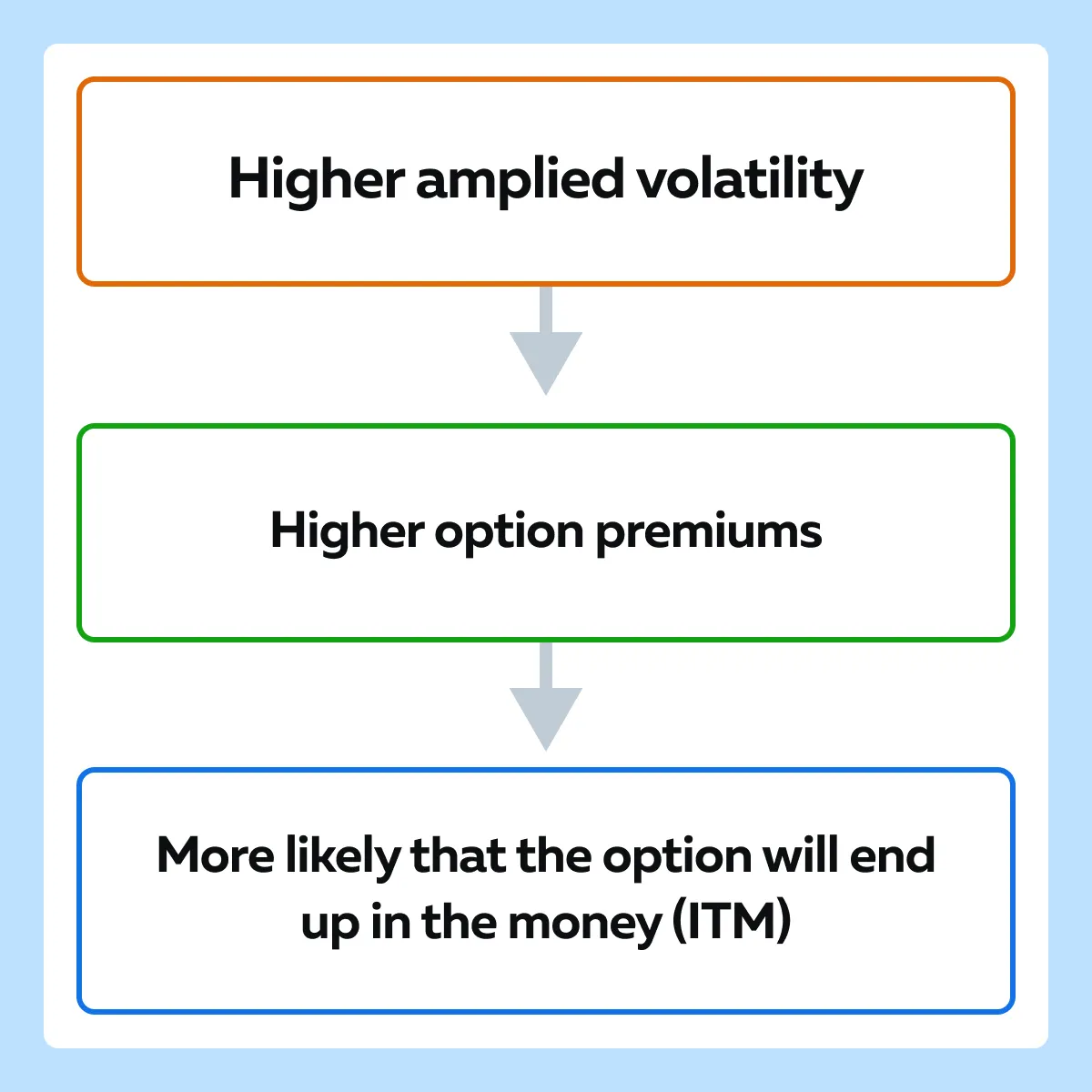
• • When implied volatility rises, the time value of options increases.

• This surge in time value leads to higher premiums.

 

• In the market, this kind of situation happens because greater expected volatility enhances the probability that the option will be profitable by expiration.

To better understand the impact of a sudden increase in implied volatility on option premiums, let’s study a hypothetical example:

• Consider an option trader, who is trading options on XYZ Corp, a tech company.
• The trader holds a call option with a strike price of $100, expiring in one month.
• The current price of XYZ Corp’s stock is $95, and the implied volatility is 20%.

 

Normal conditions

• Under normal conditions, with an implied volatility of 20%, the premium for the call option is $3.
• The trader expects XYZ Corp’s stock to rise above $100 before expiration, making the option profitable.

Sudden Increase in Implied Volatility

• Unexpectedly, XYZ Corp announces a significant product launch.
• This leads to speculation about a substantial price increase.
• As a result, the implied volatility spikes to 40%.
• With the increased implied volatility, the time value of the option rises.
• Using the Black-Scholes or a similar options pricing model, the new premium for the call option is now $6.

Impact on Trader’s Strategy

• Higher Premium: The sudden increase in the option premium presents both opportunities and challenges for the trader.
• Selling the Option: If the trader decides to sell the option, they can do so at a higher price, realizing an immediate profit from the increased premium.
• Buying New Options: However, if the trader plans to buy more options, they will now have to pay a higher price, increasing their cost and potential risk.

Strategic Adjustments

The trader might need to adjust their strategy based on the higher implied volatility. They have to:

• Consider additional hedging strategies to protect against unexpected price movements.
• Implement spread strategies like straddles or strangles, which can capitalize on increased volatility.

Historical Volatility vs. Implied Volatility: A Comparison 

Volatility arbitrage is a trading strategy. It exploits the differences between:

• Historical volatility (HV) 

and

• Implied volatility (IV).

 

Traders who engage in volatility arbitrage seek to profit from the discrepancy between an asset’s past price volatility and the market’s expectations of future volatility as reflected in options prices. Let’s understand the execution better through an example:

• Consider a trader looking to exploit volatility discrepancies for XYZ Corp, a tech company.
• They execute a volatility arbitrage strategy using these steps:

Step I: Historical Volatility Analysis: The trader calculates XYZ Corp’s historical volatility over the past 30 days and finds it to be 15%.

Step II: Implied Volatility Analysis: The trader observes that the implied volatility of XYZ Corp’s at-the-money call options is 25%.

Step III: Assess Market Sentiment: The trader believes that the market is overestimating future volatility based on upcoming events (e.g., no significant news expected).

Step IV: Short Options Position: 

• The trader decides to sell (write) options.
• They expect the implied volatility to decrease and converge towards the historical volatility.
• They sell at-the-money call options, which are currently overpriced.

Step V: Monitor and Adjust:

• The trader monitors the positions.
• They watch for changes in market conditions that affect implied volatility.

Step VI: Profit Realization:

• If the market’s implied volatility decreases as expected, the price of the options will fall
• At this time, the trader can:
  • Buy back the options at a lower price 

and

• Lock in the profit from the difference.

Let’s put numbers into the above steps for more clarity:

• Initial Trade: The trader sells 10 call options at an IV of 25%, collecting a premium of $5 per option.
• Market Adjustment: 
  • After a week, market conditions calm.
  • The implied volatility drops to 18%.
  • The price of the call options decreases to $3.
• Closing the Trade: 
  • The trader buys back the 10 call options at $3 each.
  • By doing so, they realize a profit of $2 per option (total profit: $2 x 10 = $20).

How to Use Straddle and Strangle Strategies?

Traders also use options strategies like straddles and strangles to profit from high implied volatility. They particularly execute this strategy when anticipating significant price movements regardless of direction. Let’s study both these strategies in detail:

1. A) The Straddle Strategy

A straddle involves buying both a call option and a put option with the same strike price and expiration date. This strategy profits if the underlying asset experiences significant price movement in either direction.

Let’s learn the execution of this strategy using a hypothetical scenario related to earnings announcement:

• Setup
  • A trader anticipates that XYZ Corp’s upcoming earnings announcement will cause a significant price movement.
  • However, they are unsure of the direction.
  • XYZ Corp’s stock is currently trading at $100.
• Trade Execution:
  • Buy Call Option: Strike price $100, premium $4.
  • Buy Put Option: Strike price $100, premium $3.
  • Total Cost: $7 per share (for both options).
• The Likely Outcomes:
  • Significant Price Increase: If XYZ Corp’s stock rises to $110, the call option is worth $10, and the put option expires worthless.
    • Profit: Call option value $10 – total cost $7 = $3 per share.
  • Significant Price Decrease: If XYZ Corp’s stock drops to $90, the put option is worth $10, and the call option expires worthless.
    • Profit: Put option value $10 – total cost $7 = $3 per share.
  • Little Movement: If XYZ Corp’s stock remains around $100, both options expire worthless, and the trader loses the premium paid ($7 per share).

1. B) The Strangle Strategy

A strangle involves buying a call option and a put option with different strike prices but the same expiration date. This strategy also profits from significant price movements but is cheaper than a straddle. Again, let’s learn the execution of this strategy using a hypothetical scenario related to earnings announcement:

• • Setup
    • A trader expects XYZ Corp’s stock to move significantly.
    • However, they want to reduce the cost compared to a straddle.
    • XYZ Corp’s stock is trading at $100.
  • Trade Execution:
    • Buy Call Option: Strike price $105, premium $3.
    • Buy Put Option: Strike price $95, premium $2.
    • Total Cost: $5 per share (for both options).

• The Likely Outcomes:

• Significant Price Increase: If XYZ Corp’s stock rises to $110, the call option is worth $5, and the put option expires worthless.

• Profit: Call option value $5 – total cost $5 = breakeven

• Significant Price Decrease: If XYZ Corp’s stock drops to $90, the put option is worth $5, and the call option expires worthless.

• Profit: Put option value $5 – total cost $5 = breakeven

• Little Movement: If XYZ Corp’s stock remains around $100, both options expire worthless, and the trader loses the premium paid ($5 per share). 

 

 

Managing Risk with Volatility Metrics 

Volatility metrics help traders in:

• Managing risk 

and

• Determining appropriate position sizes.

 

By understanding the historical and implied volatility of an asset, traders can balance potential returns with acceptable risk levels. It is pertinent to note that:

• Higher volatility indicates greater potential for price swings.
• Thus, it necessitates careful position sizing to avoid significant losses.

Let’s learn how to adjust position size based on historical volatility:

Consider a trader dealing with commodity futures, specifically crude oil contracts. The trader examines the historical volatility of crude oil over the past 60 days and finds that it has been highly volatile, with a standard deviation of 2%. Say the initial position size was 100 contracts.

 

• Now, given this high historical volatility, the trader decides to reduce their position size to 50 contracts to mitigate potential losses.
• If the historical volatility were low, say 0.5%, the trader might feel comfortable increasing their position size to 150 contracts. 

How to Set Stop-Loss and Take-Profit Levels?

Most traders use volatility metrics to set optimal stop-loss and take-profit levels. These levels help traders:

• Limit potential losses 

and

• Lock in profits by automatically closing positions when prices reach predefined points.

For example, say a trader who has purchased call options on XYZ Corp. They anticipate a significant price movement due to an upcoming product launch. The trader uses implied volatility to set stop-loss levels.

Initial Trade Setup

• Option Details
  • The trader buys call options with a strike price of $100, currently trading at $5.
  • The implied volatility is 30%.
• Market Expectation
  • The high implied volatility suggests significant price movements.

Setting Stop-Loss Levels

• Implied Volatility Calculation
  • The trader calculates the expected price range based on implied volatility.
  • With a 30% IV, the expected one-standard deviation move (over the option’s time frame) might be ±$10.
• Stop-Loss Level
  • The trader sets a stop-loss level below the expected range to account for potential adverse price movements.
  • For example, 
    • Say XYZ Corp’s current price is $95.
    • Now, the trader set the stop-loss at $90 to avoid excessive losses.
• Take-Profit Level
  • Conversely, the trader sets a take-profit level above the expected range to lock in gains.
  • For example,
    • Say the expected move is up to $110.
    • Now, the take-profit might be set at $115.

Managing the Trade

• Monitoring Volatility
  • The trader continuously monitors implied volatility.
  • They adjust the stop-loss and take-profit levels as necessary.
  • If IV increases, indicating even more significant expected price swings, the trader widens the stop-loss to $85 and the take-profit to $120.
• Automatic Execution
  • Using these volatility-informed levels, the trader employs automatic stop-loss and take-profit orders to manage risk effectively.
  • This automatic execution ensures the position is closed if prices move significantly in either direction.

Conclusion 

Historical and implied volatility are crucial for effective trading. While the former helps traders assess past market behavior and adjust their strategies accordingly, the latter provides insights into market expectations and influences option pricing.

 

Using these volatility metrics, traders can manage risk, determine appropriate position sizes, and set effective stop-loss and take-profit levels. This balanced approach maximizes returns while minimizing potential losses. For more tips and strategies on trading during volatile times click here.